Code
# Import necessary libraries
library(terra)
library(sf)
library(here)
library(tmap)
library(tidyverse)In the growing world of aquaculture, knowing where a species will thrive is vital. The subsequent analysis aims to determine which areas of the west coast of the United States are the best suited for a variety of aquaculture species. This is done through the utilization of spatial raster and vector data as well as species-specific requirements.
The two main requirements that this analysis takes into consideration is depth and temperature (using sea surface temperature as a proxy), as many marine species can only thrive in certain conditions. Our area of interest is split into zones in order to rank which stretches of the coastline are best and worst suited to house certain species.
This sort of analysis is significant in the face of the growing global population and climate change, which has placed a strain on agriculture worldwide. Aquaculture has been growing for years, and expanding development in a thoughtful and sustainable way could contribute to more efficient food production. More production increases food security, as well as contributes to economic growth within communities (Subasinghe et al. 2009).
In this blog post you will find an example analysis based on oysters, as well as the creation of a function that takes temperature and depth as arguments and can locate where those conditions are true.
Complete code for this analysis can be found in the corresponding Github repository.
# Import necessary libraries
library(terra)
library(sf)
library(here)
library(tmap)
library(tidyverse)Sea Surface Temperature
This analysis will use the average sea surface temperature (SST) in degrees Celsius from the years 2008 to 2012. The data was originally generated from NOAA’s 5km Daily Global Satellite Sea Surface Temperature Anomaly v3.1.
Each year of SST exists in its own raster file. In order to read them in at the same time, I created a for loop based on their standardized naming convention. It is also possible to simultaneously load in and stack multiple raster files using the rast() function, but I preferred the for loop method in my workflow!
# Create a vector of the years we have rasters for (what we will iterate over)
years <- c(2008, 2009, 2010, 2011, 2012)

# Initialize empty vectors for for loop
raster_names <- c()
file_paths <- c()

# for loop follows the following steps:
#   - iterates over the sequence in years vector
#   - for each year, creates a variable name including the year
#   - for each year, creates a file path
#   - assigns the variable name to the raster, which is read in via the created file path
for (i in seq(years)){
  raster_names[i] <- paste0("sst_", years[i])
  file_paths[i] <- paste0("blog/aquaculture-suitability/data/average_annual_sst_", years[i], ".tif")

  assign(raster_names[i], rast(here(file_paths[i])))
}

# Create raster stack (would throw error if extent, CRS, or resolution don't match)
sst <- c(sst_2008, sst_2009, sst_2010, sst_2011, sst_2012)

## Finding mean of SST

# mean() operation on raster of multiple layers creates object with one raster layer
mean_sst <- mean(sst)

# Subtract 273.15 (conversion from K to C) from all pixels
mean_sst_c <- mean_sst - 273.15
Bathymetry
Bathymetry, or ocean depth data, is provided in meters from the General Bathymetric Chart of the Oceans (GEBCO). It exists as one raster.
# Use terra package to load in raster
depth <- rast(here("blog/aquaculture-suitability/data/depth.tif"))
Exclusive Economic Zones
An Exclusive Economic Zone (EEZ) is “an area of coastal water and seabed within a certain distance of a country’s coastline, to which the country claims exclusive rights for fishing, drilling, and other economic activities” (Oxford Languages).
Our EEZ data is specifically for the west coast of the United States and comes from Marineregions.org, and contains polygons delineating each of the five zones.
# Use stars package to load in shape data frame
# quiet = TRUE argument removes output/message
eez <- st_read(here("blog/aquaculture-suitability/data/wc_regions_clean.shp"), quiet = TRUE)In order to properly perform analyses using all of data sets, we need to ensure that all three having matching CRSs. With our raster data (depth and sst), it is also necessary to confirm they have the same extent, resolution, and position. This is because our next step will be to stack them, as that raster stack is what we will be using to create a suitability mask for our species of choice.
To handle differences in the extent, we can crop depth to match sst. And to fix the issue of mismatched resolutions, we can re-sample the depth data to match the resolution of sst.
Re-sampling is the method by which we can compute values for new pixel locations in depth based on custom resolutions and origins. We will use the “nearest neighbor approach”, a technique in which the value of each cell in the output raster (in this case, depth_cropped) is calculated using the value of the nearest cell in the input raster (mean_sst) (ESRI GIS Dictionary). This fills in the new cells that will be created in order for depth to match the resolution of sst.
Finally, a way to know if we have succeeded in matching the extent, resolution, and position of our two rasters is by seeing if they will stack or not. If they do not completely match, an error will be thrown and stacking will fail.
## Matching CRSs

# Project depth raster to match CRS of sst raster
depth <- project(depth, crs(sst))

# Project (using the stars package) to match the CRS of sst raster
eez <- st_transform(eez, crs(sst))

# Crop depth raster to limits of sst raster
depth_cropped <- crop(depth, y = mean_sst_c)

# Resample depth data to match specifications of sst data, specifying nearest neighbor method
depth_cropped_resampled <- resample(depth_cropped, y = mean_sst_c, method = "near")

# Stack rasters and confirm that extent, resolution, and position all match!
depth_sst <- c(depth_cropped_resampled, mean_sst_c)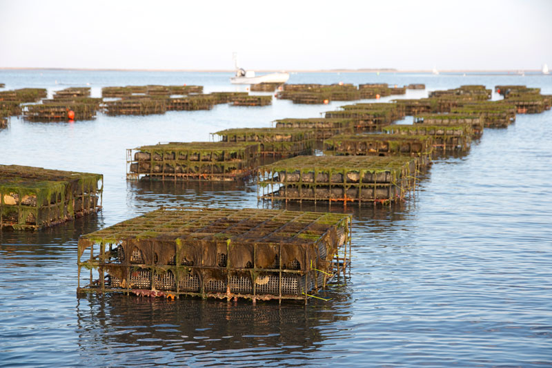
Research has shown that oysters need the following conditions for optimal growth:
These specifications can be retrieved from resources such as SeaLifeBase.
In order to find the areas with suitable growing conditions for oysters, we will assign a value of 1 to each pixel that is within the suitable range and 0 otherwise, for both of our separate raster layers.
Then, to create one suitability layer that contains suitability based on both variables, we will multiply the two layers, obtaining the following results:
This can be true because anything multiplied by 0 (not suitable in this case), will equal 0. If at least one of our layers contains 0, our new suitability layer will also contain the value 0. Cells that are suitable for both SST and depth will be the only ones that contain 1 as their value.
# Change layer names to be more indicative ("mean" --> "sst_mean")
names(depth_sst) <- c("depth", "sst_mean_c")

# Create copy of data frame to serve as mask
depth_sst_mask <- depth_sst

# Create suitability matrix based on min and max sst
sst_suitability <- matrix(c(-Inf, 11, 0,  # Will return 0 for values (-Inf, 11)
                          11, 30, 1,      # Will return 1 for values (11, 30)
                          30, Inf, 0),    # Will return 0 for values (30, Inf)
                          nrow = 3, byrow = TRUE)

# Classify sst layers using matrix
depth_sst_mask[["sst_mean_c"]] <- classify(depth_sst_mask[["sst_mean_c"]], rcl = sst_suitability)

# Create suitability matrix based on min and max sst
depth_suitability <- matrix(c(-Inf, -70, 0,
                              -70, 0, 1,
                              0, Inf, 0),
                            nrow = 3, byrow = TRUE)

# Classify depth layers using matrix
depth_sst_mask[["depth"]] <- classify(depth_sst_mask[["depth"]], rcl = depth_suitability)

# Multiply two layers and save as a new raster
oyster_suitability <- depth_sst_mask[["depth"]] * depth_sst_mask[["sst_mean_c"]]

# Rename raster layer to be more indicative ("depth" --> "suitable")
names(oyster_suitability) <- c("suitable")We want to determine the total suitable area within each EEZ in order to rank zones by priority.
This requires three distinct steps:
Find the number of cells within each zone that are deemed suitable (based on previous analysis).
Find the physical area that each cell represents (in km^2).
Multiply number of cells by area that cells represent to get actual suitable area, by zone.
We can find the number of suitable cells in each EEZ region by using the terra::zonal function. It summarizes values of one SpatRaster based on the zones provided by another. In our case, we will be summing the values of our suitable cells grouped by EEZ.
Summation works to provide the number of suitable cells in this case because we had populated suitable with “1”s and unsuitable with “0”s.
# Create a raster of species suitability only within the EEZ boundaries
suitable_westcoast <- mask(oyster_suitability, eez)

# Rasterize EEZ (will allow for zonal operations)
eez_rast <- rasterize(eez, suitable_westcoast,
                      field = "rgn")      # Set region as the value we want populating the EEZ raster

# Find the number of suitable cells per EEZ region
suitable_per_region <- zonal(suitable_westcoast, eez_rast, fun = "sum", na.rm = TRUE)
Results:
| EEZ | # of Suitable Cells |
|---|---|
| Central California | 238 |
| Northern California | 11 |
| Oregon | 71 |
| Southern California | 211 |
| Washington | 162 |
From these results, we find total suitable area within each region by multiplying the number of cells by the real-life area that each cell represents. And since we want to produce a map of West Coast EEZs colored by amount of suitable species area in each region, our final step would be to join our EEZ geometries to the data frame containing suitable area in kilometers.
# cellSize() returns a SpatRaster object of information, we want to extract just cell area
cell_area <- cellSize(suitable_westcoast, unit="km")[1]

# Multiply by each region by adding and specifying columns to data frame
suitable_per_region <- suitable_per_region %>%
  mutate(cell_area = cell_area,
         area_suitable = suitable * cell_area) %>%
  relocate(cell_area, .after = suitable)

# Join EEZ data frame (with geometries) to data frame with suitable area by region
eez_suitability_geom <- left_join(eez, suitable_per_region, by = "rgn")
The visualization of this analysis is the subsequent map of EEZ regions colored by amount of suitable area. For this, we use our original depth raster to provide a background image (and general outlines of the California coast), overlaid with the 5 West Coast EEZs, colored by amount of suitable area.
# Turn off autoscale -- messes with font size
tmap_options(component.autoscale = FALSE)

# Create map using tmap
tm_shape(depth) +                                      # Plot depth raster as first layer
  tm_raster(col.scale  = tm_scale(values = c("steelblue", "#84d18d")),
            col.legend = tm_legend(show = FALSE)) +    # Hide depth legend because not of interest
tm_shape(eez_suitability_geom) +                       # Plot EEZ polygons
  tm_polygons(fill = "area_suitable",                  # Fill by suitable area
              fill.scale = tm_scale(values = "brewer.yl_or_rd"),
              fill.legend = tm_legend(title = "Suitable Area (km²)"),
              fill_alpha = 0.6,
              lwd = 0.5) +
  tm_text(text = "rgn",                                # Add EEZ zone labels
          size = 0.7,
          xmod = -2.2,
          col = "black",
          fontface = "bold") +
tm_title("Suitability of West Coast EEZs for Oyster Aquaculture",
         size = 1)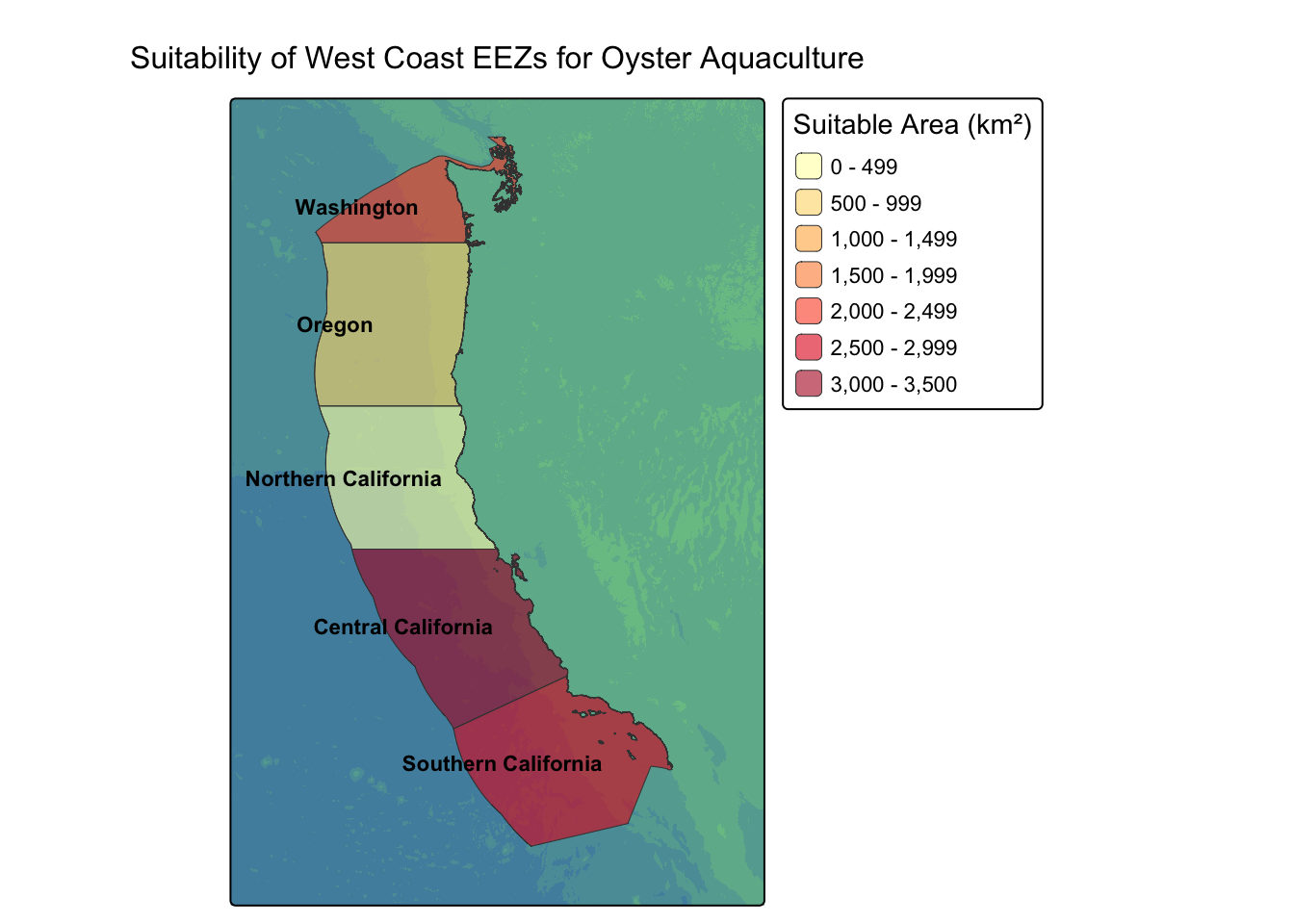
From our map, we can see that – based on suitable depth and sst – Central and Southern California are the best suited for oyster aquaculture compared to the other EEZs of the US West Coast.
In the code above, we developed a method of extracting the most suitable regions for marine aquaculture based on just a few parameters: temperature range and depth range. By making our workflow generalizable, we can create a function that takes a handle of arguments and produces a map of suitable West Coast EEZs for any marine species.
Our function will assume that the datasets/rasters sst (single layer), depth, and eez are pre-loaded and contain the correct attributes.
The other thing to note is that when inputting minimum and maximum depth, we will input the absolute value of depth (so, no negatives), with the larger number being maximum depth. For example, a depth of 70 meters, or 70 meters below sea level, should be entered as 70.
# Initialize function
west_coast_suitability_map <- function(species, min_sst, max_sst, min_depth, max_depth){

# Creating depth and sst mask based on min and max values
depth_sst_mask <- depth_sst

# sst matrix and classification, using function arguments
sst_suitability <- matrix(c(-Inf, min_sst, 0,
                          min_sst, max_sst, 1,
                          max_sst, Inf, 0),
                          nrow = 3, byrow = TRUE)

depth_sst_mask[["sst_mean_c"]] <- classify(depth_sst_mask[["sst_mean_c"]], rcl = sst_suitability)

# depth matrix and classification
depth_suitability <- matrix(c(-Inf, -max_depth, 0,
                              -max_depth, min_depth, 1,
                               min_depth, Inf, 0),
                               nrow = 3, byrow = TRUE)

depth_sst_mask[["depth"]] <- classify(depth_sst_mask[["depth"]], rcl = depth_suitability)

# Creating suitability raster
suitability_raster <- depth_sst_mask[["depth"]] * depth_sst_mask[["sst_mean_c"]]

# Renaming raster layer value to be more accurate
names(suitability_raster) <- c("suitable")

# Create a raster of species suitability only within the EEZ boundaries
suitable_westcoast <- mask(suitability_raster, eez)

# Rasterize EEZ (will allow for zonal operations)
eez_rast <- rasterize(eez, suitable_westcoast,
                      field = "rgn")      # Set region as the value we want populating the EEZ raster

# Find the number of suitable cells per EEZ region
suitable_per_region <- zonal(suitable_westcoast, eez_rast, fun = "sum", na.rm = TRUE)

# cellSize() returns a SpatRaster object of information, we want to extract just area
cell_area <- cellSize(suitable_westcoast, unit="km")[1]

# Multiplying by each region by adding and specifying columns to data frame
suitable_per_region <- suitable_per_region %>%
  mutate(cell_area = cell_area,
         area_suitable = suitable * cell_area) %>%
  relocate(cell_area, .after = suitable)

# Join eez data frame (with geometries) to data frame with suitable area by region
eez_suitability_geom <- left_join(eez, suitable_per_region, by = "rgn")

# Turn off autoscale -- messes with font size
tmap_options(component.autoscale = FALSE)

# Create map using tmap
suitability_map <- tm_shape(depth) +                                      # Plot depth raster as first layer
  tm_raster(col.scale  = tm_scale(values = c("steelblue", "#84d18d")),
            col.legend = tm_legend(show = FALSE)) +    # Hide depth legend because not of interest
tm_shape(eez_suitability_geom) +                       # Plot EEZ polygons
  tm_polygons(fill = "area_suitable",                  # Fill by suitable area
              fill.scale = tm_scale(values = "brewer.yl_or_rd"),
              fill.legend = tm_legend(title = "Suitable Area (km²)"),
              fill_alpha = 0.6,
              lwd = 0.5) +
   tm_text(text = "rgn",                                # Add EEZ zone labels
          size = 0.7,
          xmod = -2.2,
          col = "black",
          fontface = "bold")+
tm_title(paste("Suitability of West Coast EEZs for", species, "Aquaculture"),
         size = 1)

return(suitability_map)
}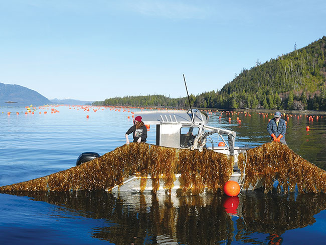
Bull kelp farming is a niche sector of seaweed aquaculture, especially small compared to the large seaweed operations taking place in Asia. Currently, there are only a few active, albeit experimental, bull kelp farms in Alaska and BC.
This lack of development is partially due to the fact that bull kelp is not necessarily a commercial commodity in the same way other species of seaweed, such as sugar kelp (Sacharrina latissima) or ribbon kelp (Alaria marginata), are. Despite its challenges, bull kelp is essential for ocean health and biodiversity, so farming more of it could help with restoration efforts, as well as help fill knowledge gaps in its cultivation.
Bull kelp’s suitability conditions are as follows:
# Use function to plot regions with highest suitability
west_coast_suitability_map(species = "Bull Kelp" ,
                           min_sst = 10,
                           max_sst = 16,
                           min_depth = 40,
                           max_depth = 17)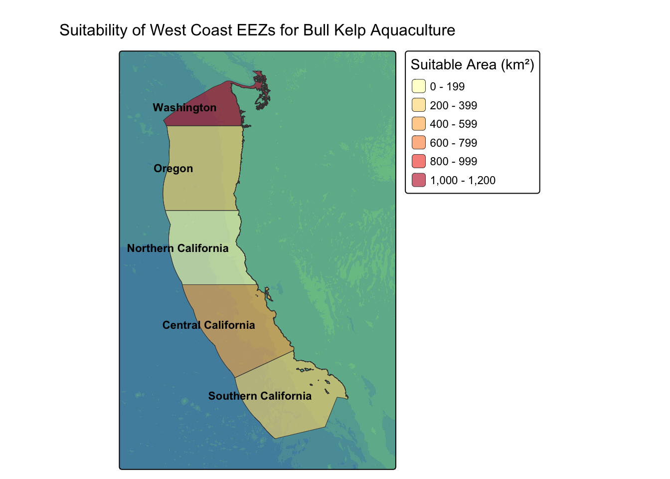
From this visualization, we can see that – based on suitable depth and sea surface temperature – the Washington region is by far the best suited for bull kelp aquaculture compared to the other EEZs of the US West Coast. This agrees with our previous research: if successful bull kelp farms are mostly in Alaska and Canada, it would make sense that the northernmost region would be the most suitable.
This blog post used packages such as terra and sf to combine raster and vector data on ocean depth and temperature, and classify different zones along the cost based on specifications. In our case, we were able to determine that the southern California coast is the most suitable for oyster aquaculture whereas the northern coast – specifically the Washington EEZ – is best for bull kelp.
It is important to note, however, that sea surface temperature and depth are only two of the many factors that influence aquaculture success. Our analysis not only excludes other variables such as current strength, salinity, and water quality, but also fails to consider future changes to ocean temperature that may be crucial in the planning of aquaculture.
Despite these caveats, this sort of code is generalizable first step to a variety of uses that involve finding most suitable areas – not just for aquaculture. And especially with the creation of a function, the possibilities are endless.
California Department of Fish and Wildlife, Marine Species Portal. (n.d.). Kelp and other marine algae — True kelp species in California. Accessed November 20, 2025. https://marinespecies.wildlife.ca.gov/kelp/true/#:~:text=Bull%20kelp%20grows%20on%20similar,and%20on%20wave%2Dexposed%20reefs
Subasinghe, R., Soto, D., & Jia, J. (2009). Global aquaculture and its role in sustainable development. Reviews in aquaculture, 1(1), 2-9.
The Mysterious World of Bull Kelp. (n.d.). Aquaculture. Accessed November 20, 2025. https://bullkelp.info/aquaculture
Weigel, B. L., Small, S. L., Berry, H. D., & Dethier, M. N. (2023). Effects of temperature and nutrients on microscopic stages of the bull kelp (Nereocystis luetkeana, Phaeophyceae). Journal of phycology, 59(5), 893–907. https://doi.org/10.1111/jpy.13366